



Download the “Agentic AI” e-book for free

AWS isn’t winning the AI race with the smartest model. It’s winning by owning everything that surrounds the model. Six layers. Sixty-plus services.
But how do you actually put all those pieces together?
AWS asked 15+ data and AI leaders from companies including PayPal, Siemens, Morgan Stanley, and Sanofi how they are approaching agentic AI in the enterprise.
The result is The Agentic Enterprise: a 16-chapter e-book covering practical topics such as:
Building, monitoring, and governing reliable AI agents
Improving agent performance and scalability
Implementing guardrails throughout the AI lifecycle
Moving agentic systems toward production
If you’re working on AI agents beyond the prototype stage, it’s worth a read.
Download the e-book for free here »
(Thanks to AWS for partnering on this newsletter.)
Imagine you’re building Shazam1.
A user hums a 10-second song clip…Your system has 100 million songs.
Your job is simple: find the most similar songs in less than 50 milliseconds.
So how’d you do it?
Here’s the obvious solution: compare the user’s song with each song in the database.
Query song
   ↓
Song 1
Song 2
Song 3
...
Song 100,000,000
Yet this does NOT work at scale.
Even if each comparison is fast, 100 million comparisons are “expensive”.
When you search documents in a Retrieval-Augmented Generation (RAG2) system, find similar images, or generate recommendations, the system is doing the same thing:
Find the most similar items in a massive collection.
This is where Hierarchical Navigable Small World (HNSW3) comes in…
§
Share this letter & I’ll send you some rewards for the referrals.
§
I want to introduce Avani Chaskar as the guest author.

She writes technical guides on building, evaluating & scaling deterministic AI systems.
Subscribe to her newsletter to join developers receiving her latest engineering breakdowns.
§
The Idea: Search Only What Matters
The idea behind HNSW is simple:
Instead of comparing against every item, build shortcuts that lead you close to the answer.
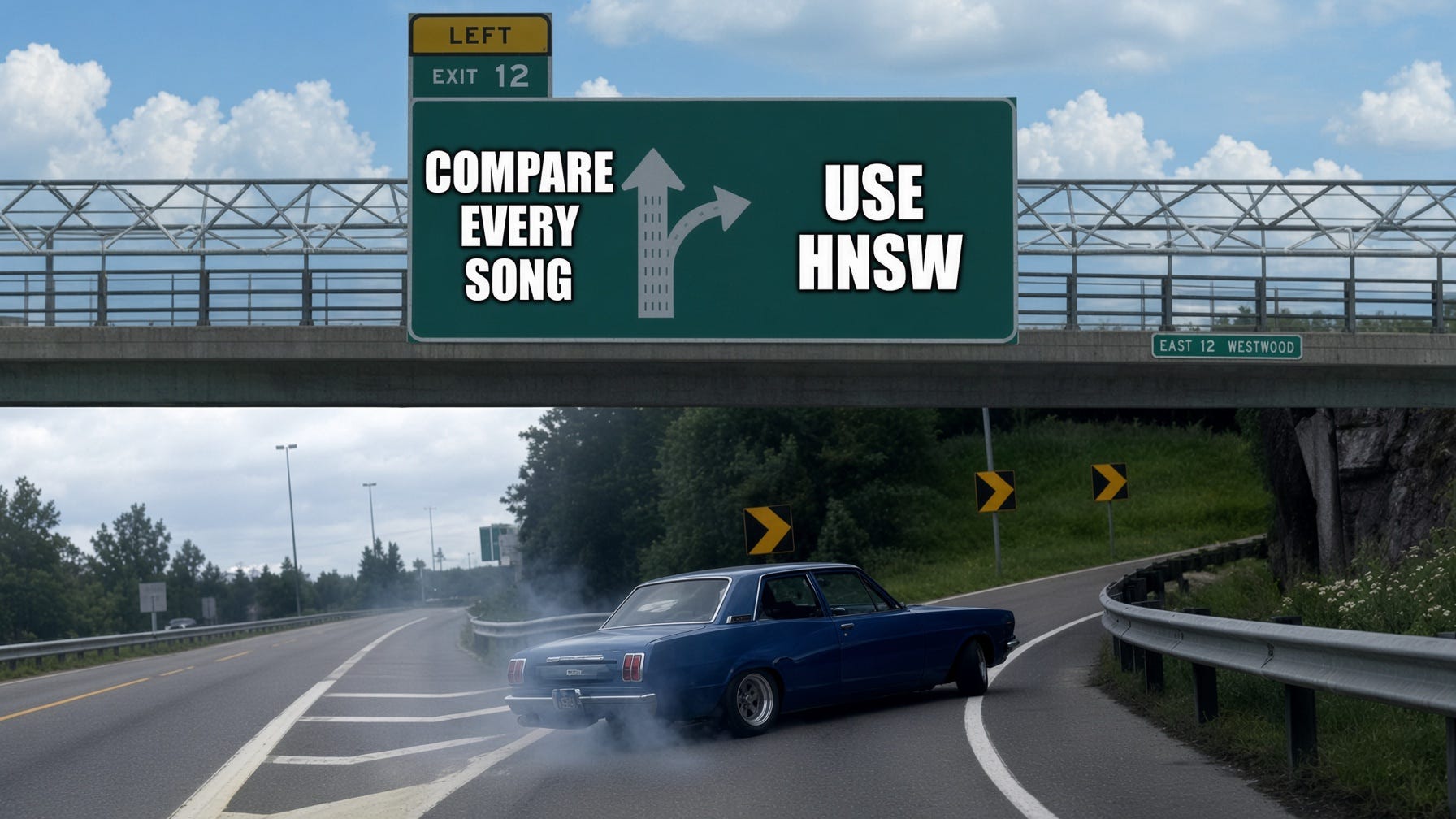
Think about finding a coffee shop in a city you do not know.
You would not walk down every street…Instead, you’d:
Use highways to reach the right area.
Take the main road to get closer.
Then use local streets to find the exact place.
§
First Attempt: Build a Graph
Let’s go back to our 100 million songs.
Suppose each song is connected to similar songs:
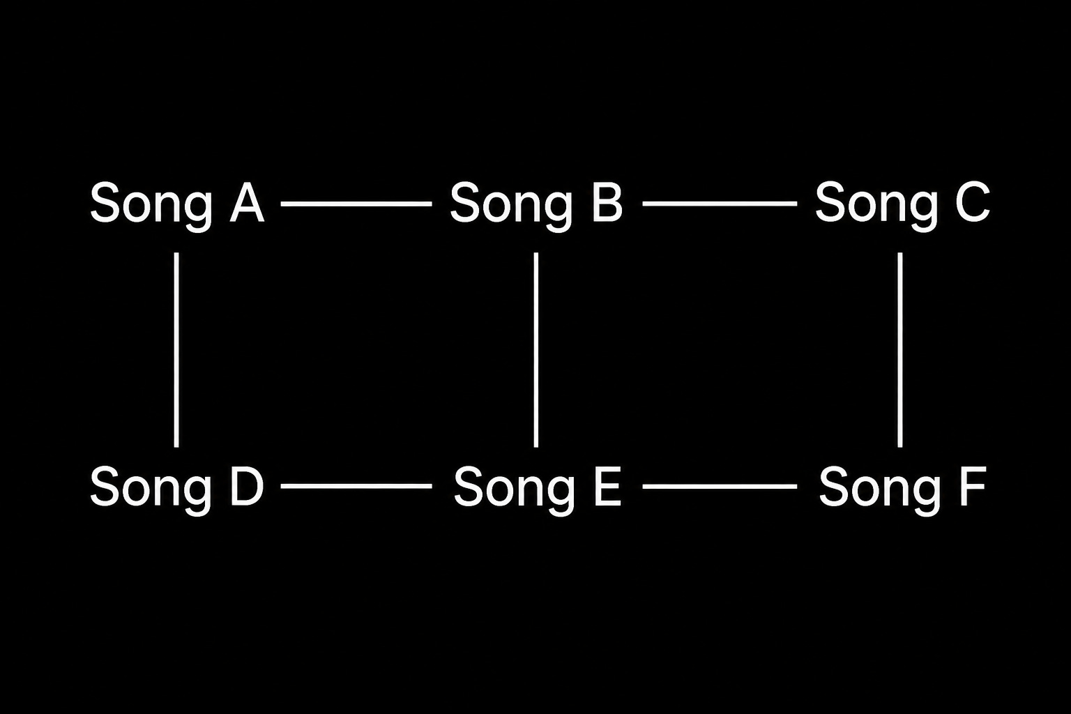
If Song B is similar to Song E, we connect them…
So instead of checking every song, we can jump from one song to another.
Start somewhere:
Move to a neighbor that is closer to the query,
Then repeat.
This is much faster!..
But there is still a problem: a graph with 100 million nodes still requires “many” hops.
i.e., we need a faster way to move…
§
But What Does “Similar” Actually Mean?
Before HNSW navigates the graph, it needs a way to measure how close two vectors4 are.
Here are the most common distance or similarity metrics:
Cosine similarity: Measures the angle between vectors. A smaller angle means higher similarity. It ignores vector length, making it ideal for text and NLP5.
Dot product/inner product: Multiplies & sums elements. A larger positive value means higher similarity (it grows with both alignment and length). It’s commonly used in recommendation systems.
Euclidean distance (L2): Measures straight-line distance. A smaller distance means higher similarity. It captures absolute size differences, making it great for images.
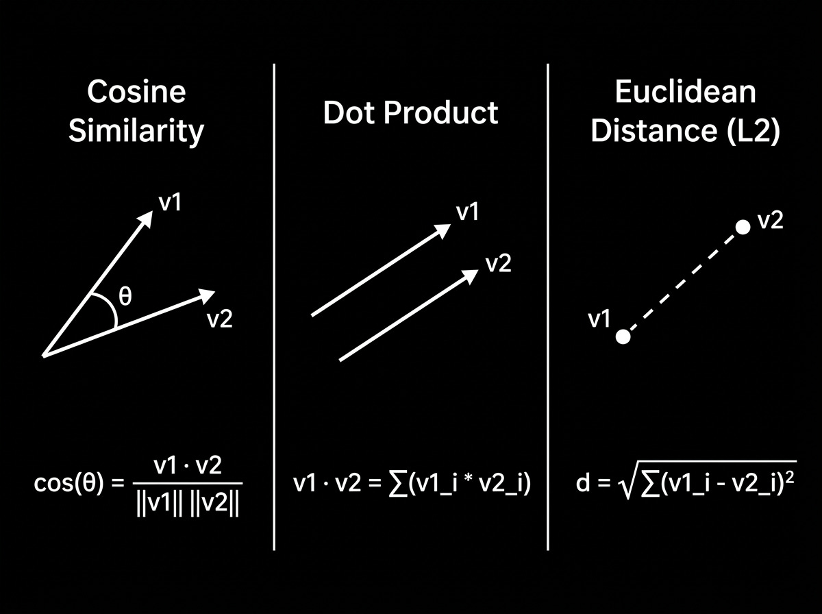
So the right similarity metric depends on the embedding model6 & use case.
For HNSW, the important idea is simple:
The closer a vector is to the query according to the chosen metric, the better the match.
§
Exact Search vs Approximate Search
There are two ways to find the nearest vectors:
Exact search: Compares the query against every vector & returns the mathematically closest results. That gives us the true nearest neighbors, but at 100 million or a billion vectors, checking everything is “expensive”.
Approximate Nearest Neighbor (ANN): Instead of examining the entire dataset, it explores the most promising clusters of the index and returns results that are very likely to be the true nearest neighbors.
HNSW is an ANN algorithm.
Yet this creates an important tradeoff:
Explore more → higher recall7, higher latency.
Explore less → lower latency, potentially lower recall.
To measure search effectiveness, we use Recall@k.
It measures how many of the true top-k nearest neighbors an approximate search actually retrieves.
HNSW gives us a way to search a tiny fraction of the dataset while still achieving high recall.
§
The Real Trick: Add Layers
This is the key idea behind HNSW:
HNSW builds many layers of graphs8.
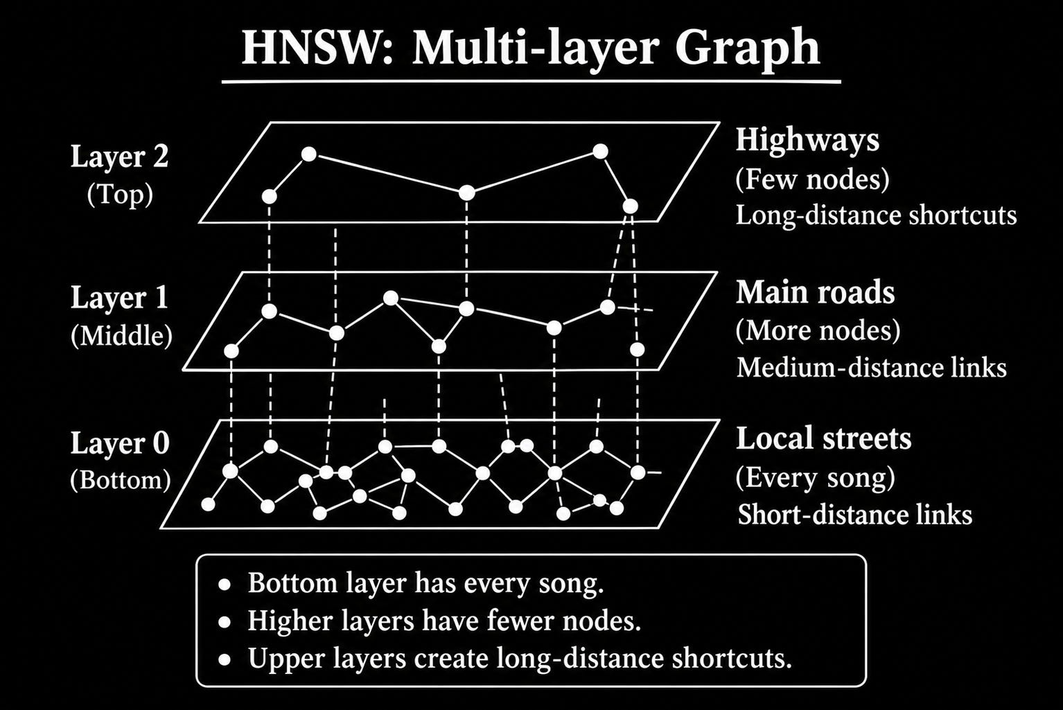
The bottom layer contains every song.
Higher layers contain fewer songs. The higher you go, the fewer nodes exist. These upper layers create long-distance shortcuts.
This makes HNSW fast!
§
How HNSW Search Works
Here’s how:
A user hums a song: the system converts it into a vector.
A vector is simply a list of numbers:
[0.12, 0.87, 0.34, 0.91, ...].Songs with similar vectors sound similar.
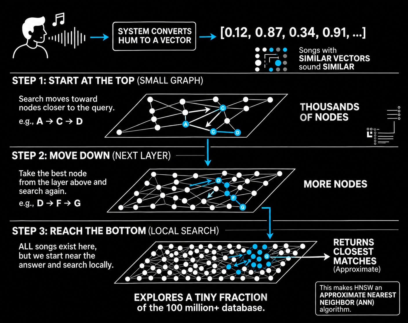
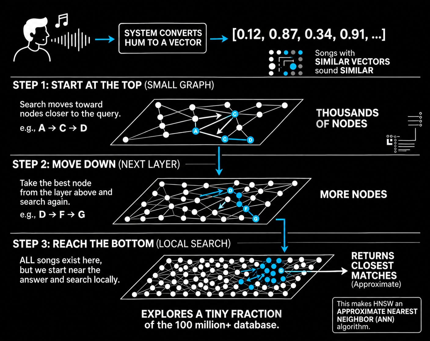
Now the search begins…
Step 1 (Top Layer): Performs a high-level traversal on a sparse graph (
A → C → D) to locate the general neighborhood rapidly.Step 2 (Middle Layers): Drops down through denser layers (
D → F → G), narrowing the distance to refine the search space.Step 3 (Bottom Layer): Executes a targeted, local search among millions of nodes- exploring only a tiny fraction of the dataset to return Approximate Nearest Neighbors.
Key Insight
HNSW does not make 100 million comparisons faster.
It avoids making 100 million comparisons in the first place.
That is the entire trick.
§
Why the “Small World” Matters
Think about social networks:
You know someone. That person knows someone else. After a few connections, you could reach almost anybody.
Graphs with this property are called small-world graphs9.
HNSW uses this idea:
Most connections are local…some connections jump far.
Together, they create short paths through huge datasets.
§
Why “Hierarchical”?
Because there are layers…
Each higher layer contains exponentially fewer nodes.
Think of it like this:
Layer 3: Highways
Layer 2: Major roads
Layer 1: Streets
Layer 0: Every location
Search starts “fast”…then becomes “precise”.
§
How Layers Get Built?
When inserting a new vector into an HNSW index:
The algorithm assigns the vector a maximum height layer based on a decaying probability distribution10.
Most vectors reside exclusively on Layer 0.
A small fraction are promoted to middle layers, and only a tiny minority reach the sparse top layer.
This is similar to a data structure called a skip list11.
Skip lists let you jump over many elements.
HNSW applies the same idea to vectors.
Randomness creates shortcuts → Those shortcuts make navigation efficient.
§
How HNSW Builds the Graph
When a new vector gets inserted, HNSW searches the existing graph to find promising neighbors.
It does NOT simply connect the new vector to the closest M vectors it happens to find. Instead, a neighbor-selection heuristic tries to keep connections useful and diverse, avoiding too many redundant links.
The process looks roughly like this:
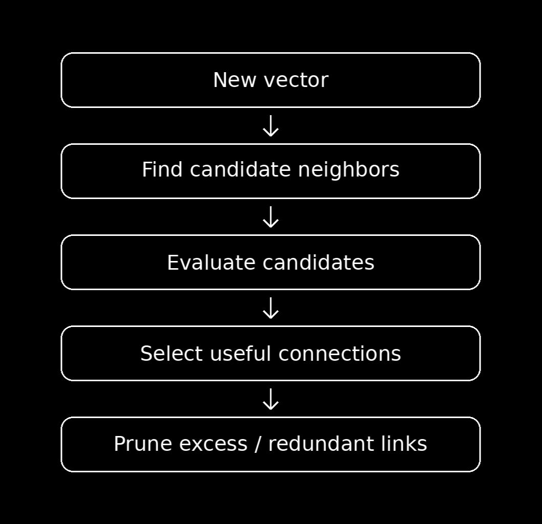
This is where efConstruction12 matters:
A higher efConstruction means the algorithm considers a larger candidate set while building the graph. That usually produces a better-connected graph, but indexing takes longer.
A lower value makes construction faster, but the resulting graph may provide fewer useful paths during search.
Good graph construction matters because graph quality directly affects both search speed & recall.
§
§
Three Knobs Engineers Tune
In production systems, these three parameters matter most:
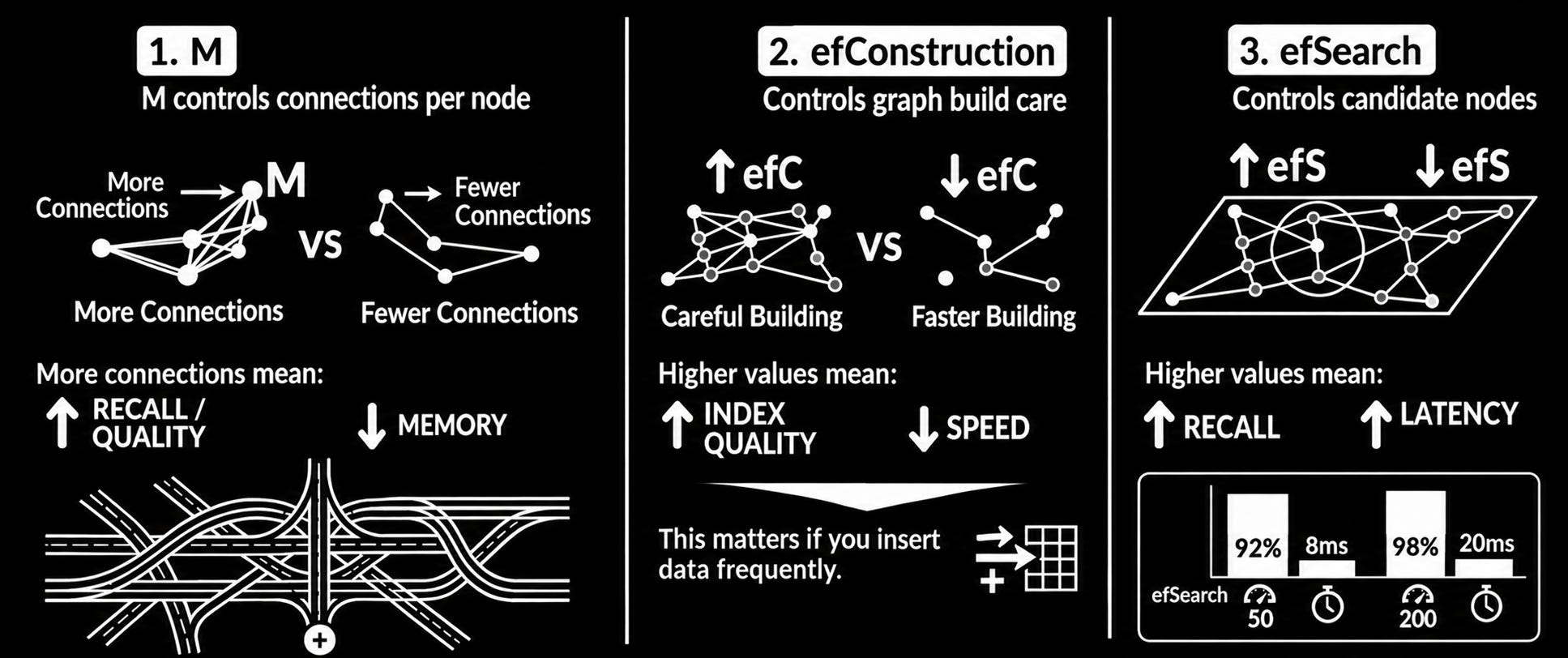
1. M
M controls how many connections each node has.
More connections mean:
Better search quality
More memory usage
Think of it as building more roads:
More roads improve navigation.
But roads are expensive.
2. efConstruction
This controls how carefully the graph gets built.
Higher values mean:
Better graph quality
Slower indexing
Lower values mean:
Faster indexing
Slightly lower search quality
This matters if you insert data frequently.
3. efSearch
This determines how many candidate nodes the system explores during the search.
Higher values mean:
Better recall
Higher latency
Lower values mean:
Faster queries
Lower recall
For example:
efSearch = 50
>Recall = 92%
>Latency = 8 ms


efSearch = 200
>Recall = 98%
>Latency = 20 ms
The exact values depend on the dataset...this is an engineering tradeoff.
§
Why HNSW Uses So Much Memory
HNSW stores:
Vectors,
Graph connections,
Metadata.
The graph itself could become large…for millions/billions of vectors, memory usage grows quickly…
So many systems combine HNSW with compression techniques such as:
Scalar Quantization (SQ8): Compresses float32 vectors down to int8, reducing RAM footprint by ~75% with minimal recall impact.
Product Quantization13 (PQ): Segments vectors into sub-vectors and quantizes them into cluster centroids, unlocking extreme memory savings for billion-scale indexes.
Key Insight
Compression reduces memory usage.
So you lose a little precision.
But you save a ton of space.
§
When to Use HNSW
HNSW is a good choice when:
Search speed matters: get results in milliseconds at large scale.
High recall matters: for the search to capture most of the truly similar results.
The dataset fits in memory: larger datasets demand more RAM, since HNSW keeps its graph in memory
Data updates are moderate: HNSW works best when vectors get added occasionally, and not constantly.
Best use cases:
RAG systems,
Image search,
Audio matching,
Semantic search,
Recommendations.
But HNSW is NOT ideal when:
Memory is very limited: Graph connections add significant RAM overhead.
Data changes constantly: Frequent updates make the graph expensive to maintain.
Exact nearest neighbors are required: HNSW is approximate, so it occasionally misses the mathematically closest match.
No algorithm is free → HNSW trades memory for speed & search quality.
§
The HNSW Mental Model
HNSW is built around one simple idea:
Don’t make the search faster…Make the search smaller.
Instead of looking at every vector, build a structure that tells you where to look.
The idea is simple…The scale it unlocks is not.
Millions of vectors. Billions of vectors. Milliseconds.
That’s the power of HNSW.
§
I’d like to thank Avani Chaskar for writing this newsletter.
She writes technical guides on building, evaluating & scaling deterministic AI systems.
Subscribe to her newsletter for more such quick reads on AI Engineering topics.
§
If you’re serious about AI engineering, you really can’t miss out on the footnotes:

Want to reach 250K+ tech professionals at scale? 📰
If your company wants to reach 250K+ tech professionals, advertise with me.
Thank you for supporting this newsletter.
You are now 250,001+ readers strong, very close to 251k. Let’s try to get 251k readers by 17 October. Consider sharing this letter with your friends & get rewards.
Y’all are the best.
