

Share this letter & I’ll send you some rewards for the referrals.
We were taught that making LLM inference faster means using more powerful GPUs.
That advice is exactly why we have expensive hardware underused while users wait longer for responses.
Here’s what works instead1:

n8n just launched a new type of AI agent, one you can control.
It works toward a goal and can act through tools like Gmail or Slack. You can also give it n8n workflows as tools that run exactly as you built them, so you decide which actions the agent handles on its own and which follow a set process. Add approvals before sensitive actions and see every action it takes.
Built for teams that need agents they can rely on.
(Thanks to n8n for partnering on this newsletter.)
Batching
Batching processes many requests together instead of running each request through the model separately.
A real AI service might have many users waiting for tokens at the same time. Processing each request separately would leave much of the GPU’s available capacity unused.
Batching allows several sequences to be processed together.
During decode2, the GPU repeatedly needs access to the model’s weights. When only one request is being processed, those weights are being used to advance only one sequence.
Imagine four users are waiting for their next token:
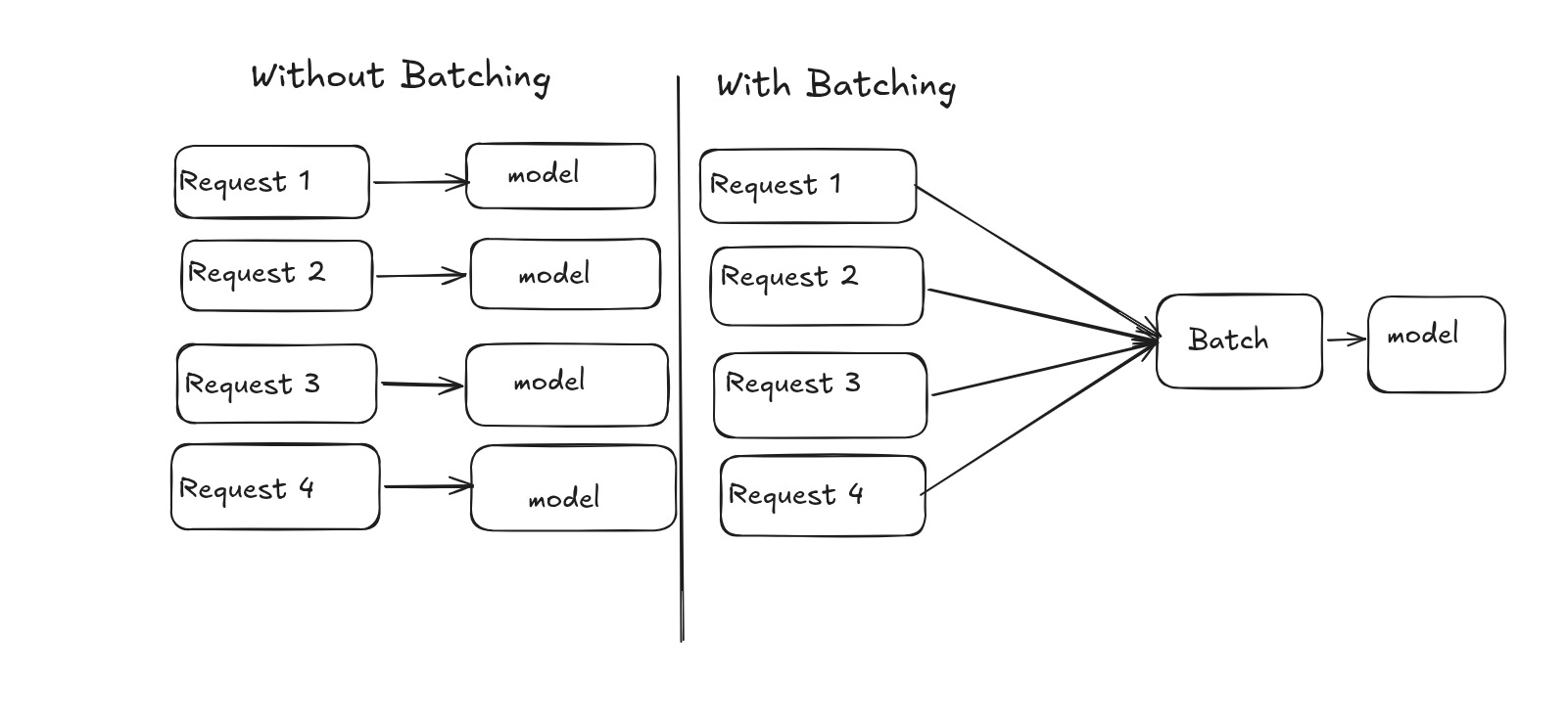
The inference system groups those requests into a “batch”.
During the next decode step, the GPU processes the current position for ALL four sequences together. The model weights are still needed, but the work done with those weights is spread across several requests. This gives the GPU more computation to perform for the data it accesses and makes better use of its parallel processing capacity.
The same idea applies to arithmetic intensity3.
Processing more sequences together increases the amount of useful computation performed while the model weights are being used. But batching does not make additional requests free.
A batch of thirty-two requests requires more computation than a single request.
Each sequence also has its own attention4 work, intermediate values, and KV cache. As the batch grows, both compute & memory usage increase. The advantage is the GPU can use its resources much more efficiently.
This introduces an important distinction between latency & throughput.
Latency describes how long an individual request takes.
Throughput describes how much total work the system can complete in a time period, typically measured in tokens per second across all requests.
Batching mainly improves throughput because the system advances many sequences together instead of one at a time.
But there are limits to how large a batch could become…Memory is one of them.
Every active request needs space for its KV cache, and the cache grows as the sequence gets longer. A large batch of long conversations could eventually consume the available GPU memory.
Timing creates another problem…
Real requests do not arrive/finish together.
Imagine four requests enter a batch:
Request A → finishes after 20 tokens
Request B → finishes after 100 tokens
Request C → finishes after 50 tokens
Request D → finishes after 200 tokens
Request A finishes much earlier than Request D.
With “static” batching, the group gets formed before processing begins. When shorter requests finish, their places are not immediately filled with new requests. So newer requests wait while the remaining requests in the current batch continue.
This reduces some of the efficiency batching was meant to provide.
Real traffic is constantly changing…
Users send prompts at different times.
Plus prompts have different lengths.
Also generated answers finish after different numbers of tokens.
i.e., an efficient serving system needs a batch that changes while the model is generating.
That’s why we need continuous batching...
Continuous Batching
Continuous batching means changing the group of requests being processed as requests finish & new ones become ready.
Imagine 32 requests starting together:
One request finishes after 20 tokens, another after 100, and another keeps generating for 500 tokens.
With static batching, the group gets decided before generation begins. Shorter requests finish while longer ones are still running. New requests then have to wait for the current batch to complete.
Continuous batching changes how the system schedules this work. (Remember, decode happens one step at a time.)
The model generates the next token for the active sequences, then moves to the next generation step. Instead of scheduling an entire request from beginning to end, the system makes scheduling decisions between these iterations.
This is called “iteration-level” scheduling.
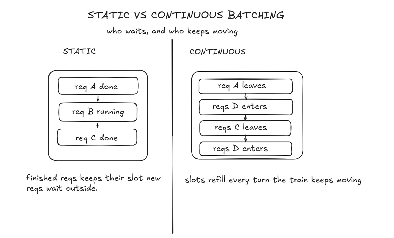
Suppose the active batch looks like this:
A B C D
After a generation step, Request A finishes.
The scheduler removes A and uses the available capacity for another waiting request when the system has enough compute and memory available.
The batch can therefore change while generation continues.
Step 1 → A B C D
Step 2 → A B C D
…
A finishes
…
Step 3 → E B C D
i.e., the system does not need to wait for B, C & D to finish before it considers E.
This makes continuous batching better suited to real traffic, where requests arrive at different times and generate answers of different lengths. The idea became important in LLM serving through systems such as Orca, which introduced iteration-level scheduling for generative Transformer models. Modern inference engines such as vLLM use continuous batching as part of their serving systems.
But adding a new request is not free/automatic.
Every active request consumes resources, including space for its KV cache. Also, the scheduler has a limit on how many sequences and tokens it can process in one iteration. A new request only joins when the system has enough capacity to schedule its work.
Besides new requests need prefill before they continue through decode.
Modern inference engines must decide how to schedule prefill work alongside requests already generating tokens.
So continuous batching is about more than filling empty slots…
The scheduler repeatedly decides which requests should use the GPU next instead of locking the GPU into one batch until every request finishes. This keeps the hardware busy even when users arrive & leave at unpredictable times.
Plus different requests could share more than the same GPU.
Many begin with the same tokens. Recomputing those tokens every time creates another unnecessary workload.
This is where you need prefix caching...
Prefix Caching
Prefix caching means reusing the KV cache for a prompt beginning the model has already processed.
Many requests sent to an AI app begin with the same tokens.
A chatbot would use the same system instructions at the beginning of every request.
A Retrieval-Augmented Generation (RAG) application would repeatedly send the same document/context before asking different questions about it.
Even a normal multi-turn conversation contains repeated text.
When you send another message, the app sends much of the earlier conversation back to the model as part of the new prompt. Without caching, the model would process those repeated tokens again during prefill.
But the KV cache could help.
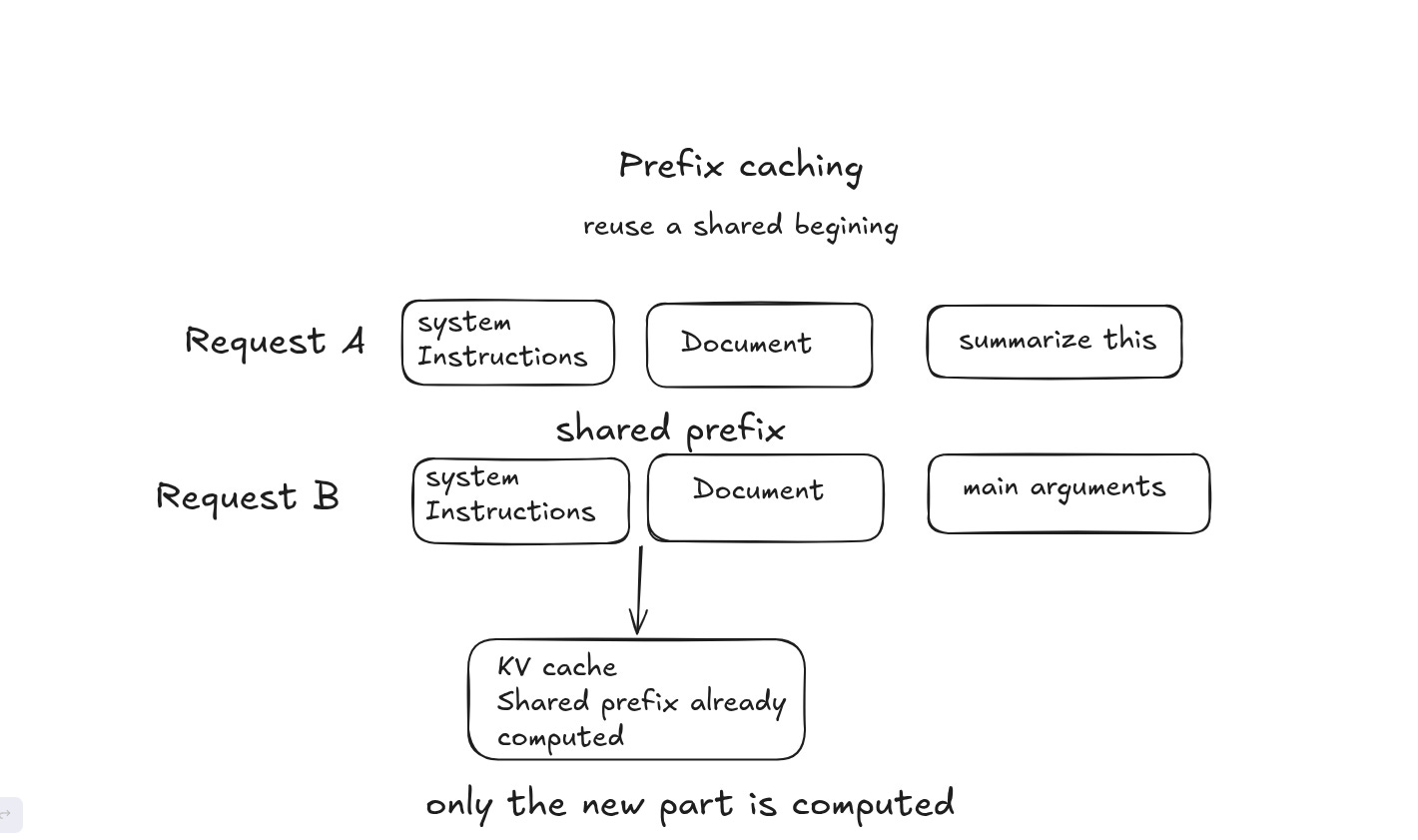
During prefill, the model computes keys & values for prompt tokens and stores them in the KV cache.
If another request begins with exactly the same sequence of tokens, the system reuses the keys and values already computed for that shared beginning.
That shared beginning is called a “prefix”.
Imagine 2 requests look like this:
Request A: [System instructions] + [Document] + “Summarize this”
Request B: [System instructions] + [Document] + “What are the main arguments?”
Both requests begin with same system instructions & document.
With prefix caching, the inference system reuses cached KV data for the matching prefix instead of recomputing it. Prefill only needs to process the part that is not already available in the cache.
The keyword here is prefix.
The matching tokens have to appear at the beginning of the request. Once the token sequence differs, later KV states depend on that different sequence and cannot simply be reused as part of the same cached prefix.
This is why prompt order matters for caching.
If an app has a large block of instructions/context that stays the same across requests, placing that stable content before the parts that change increases how much of the prompt is reusable.
Prefix caching reduces repeated prefill computation.
For long shared prefixes, this reduces time to first token because the model has fewer uncached prompt tokens to process before generation begins. Also it reduces cost when a provider charges less for cached input tokens than for uncached input tokens.
But a cached prefix does NOT make the entire request free.
Any new part of the prompt still needs processing, and output still has to go through decode.
Now many requests share the GPU, batches change while generation runs, and cached prefixes avoid repeated work.
But when more requests are waiting than the system can handle at once, the request scheduler decides which one runs next…
Request Scheduling
Request scheduling decides which requests get to use the model & when they get to run.
Continuous batching lets requests enter & leave while generation is happening.
But the GPU can only handle so much work at once…
Imagine 100 requests waiting, but the inference server currently has enough capacity to process only part of them…The remaining requests have to wait. This creates a “queue”. The scheduler sits between that queue & the model. Its job is to decide which requests move from waiting into active processing.
The simplest approach is first-come-first-served (FCFS):
The first request to arrive is considered first.
If Request A arrives before Request B, the scheduler tries to process A before B.
But arrival time is not the only way to make this decision…
Some systems also support priority scheduling. A request can be assigned a priority, and the scheduler considers higher-priority work before lower-priority work. Arrival time can then decide between requests with the same priority.
Choosing a request is only part of the scheduler’s job.
Also it has to check whether enough resources are available to run it. Every active request needs KV-cache memory, and the model also has a limit on how many sequences & tokens it can process during an iteration.
So even if a request is next in the queue, the scheduler cannot keep adding work.
Suppose the GPU is already processing several long conversations:
Their KV caches occupy most of the available cache memory. Another request is waiting... Before admitting it, the serving system has to check whether enough capacity remains.
Admitting too many requests could create memory pressure and force the system to interrupt and/or rearrange already running work.
“Admission control” decides whether new work should enter the active system based on currently available resources. The exact rules depend on the inference engine, but the goal is the same: avoid accepting more active work than the system can handle efficiently.
Scheduling therefore involves more than asking, “Who arrived first?”
The system has to balance waiting requests against available compute, token budgets & KV-cache memory.
This matters even more because the KV cache is NOT a fixed size.
Every new token makes it grow. With many active users, those caches have to share a limited amount of GPU memory. How that memory is allocated determines how many requests the server can keep running at once.
That brings us to PagedAttention…
PagedAttention
PagedAttention is a technique that manages the KV cache in small blocks instead of storing each request’s cache in one large, continuous area of GPU memory.
KV cache grows as a model processes more tokens... The problem is the inference server does NOT know exactly how large each request’s KV cache will become…
Imagine a user sends a prompt & model is allowed to generate up to 1,000 tokens:
The answer might finish after 100 tokens, or it might use almost the entire limit. One approach is to reserve enough continuous GPU memory for the maximum possible sequence length before generation begins.
But much of that reserved space could remain unused if the request finishes early.
There is another problem called “fragmentation”.
Imagine GPU memory as a row of storage spaces:
Requests enter & leave, creating free spaces in different places over time. There may be enough free memory in total for a new KV cache, but not enough “continuous” free space where the system expects to place it.
Both problems waste memory that could otherwise hold more active requests.
PagedAttention solves this by borrowing an idea from operating-system virtual memory: paging.
Instead of requiring a request's KV cache to occupy one continuous area of physical memory, PagedAttention divides it into “fixed-size” blocks.
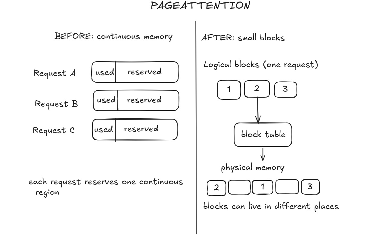
A request then uses blocks located in different places in GPU memory.
The blocks do not have to sit next to each other physically.
The system tracks their locations using a “block table”. This gives the model a logical view of the request’s KV cache while the memory manager handles where those blocks actually live.
Also more blocks could be allocated as the sequence grows…
Instead of reserving memory for a 1,000-token answer that might stop after 100 tokens, the system allocates KV-cache blocks as they’re needed.
Some unused space may remain in the final block.
A sequence does not always end exactly at a block boundary. But the amount of wasted memory is much smaller than reserving a large continuous region for every request.
This matters because KV-cache memory limits how many requests remain active on a GPU.
If each request wastes less memory, the server could keep more sequences in memory at the same time. This enables larger effective batches, thus increasing throughput.
Plus, paged blocks make sharing KV-cache data easier.
If two requests share the same cached prefix, their block tables refer to the same physical KV-cache blocks instead of storing another copy for each request. (This connects PagedAttention directly to the prefix caching.)
The original vLLM work reported near-zero waste in KV-cache memory. Also it improved throughput two to four times over the serving systems it compared against while maintaining similar latency.
PagedAttention does not make the KV cache smaller by changing what the model stores. Instead, it changes how that cache is placed and managed in memory, thus allowing the available GPU memory to be used more efficiently.
But KV-cache storage is only one part of the attention problem.
Even with efficient memory allocation, the model has to perform the attention computation itself.
This brings us to FlashAttention…
FlashAttention
FlashAttention5 is a faster way to compute attention by reducing how much data moves between different GPU memory levels.
When the model processes a sequence, each token needs a way to decide which earlier tokens are relevant. Attention does this by comparing tokens & producing scores that describe how strongly one position should attend to another.
For a sequence with 2,000 tokens, this could involve millions of attention scores.
A straightforward implementation creates a large matrix containing these intermediate scores.
The GPU writes intermediate data to its high-bandwidth memory (HBM), reads it back for another operation, writes another result, and continues through the attention calculation.
The calculations themselves are fast on a GPU.
But moving all those intermediate values between HBM & GPU’s much smaller on-chip memory would become extremely expensive.
FlashAttention changes how this calculation is performed.
Instead of computing & storing the entire attention matrix in HBM, it divides the work into smaller pieces called “tiles”. Each tile is small enough for the GPU to work on using its faster on-chip SRAM.
The GPU loads a portion of the required data, performs several parts of the attention calculation there, and combines the results without writing the full attention matrix to HBM.
This keeps more of the work close to the GPU’s compute units.
Instead of repeatedly moving large amounts of intermediate data in and out of HBM, FlashAttention reduces these expensive memory transfers.
There is an important detail here:
FlashAttention does not approximate standard attention to make it faster. It computes exact attention while changing how the computation is organized around the GPU’s memory hierarchy.
Also it does not remove the quadratic amount of arithmetic required by standard dense attention.
If the sequence length doubles, the number of token-to-token comparisons still grows roughly with the square of the sequence length. FlashAttention reduces the intermediate memory it needs and the number of expensive reads and writes to HBM.
Its auxiliary memory requirement grows linearly, not quadratically, with sequence length.
This distinction explains why FlashAttention makes exact attention much faster without changing what the attention operation computes.
The original FlashAttention work showed that paying attention to where data moves, not only how many calculations are performed, produces large speed improvements.
PagedAttention & FlashAttention therefore solve two different memory problems:
PagedAttention manages how the KV cache gets stored while serving requests.
FlashAttention improves how the attention calculation itself moves data through GPU memory.
But even an efficient algorithm still has to become instructions the GPU can execute.
Those instructions run inside GPU kernels…
Reminder: this is a teaser of the subscriber-only newsletter, exclusive to my golden members.
When you upgrade, you’ll get:
High-level architecture of real-world systems.
Deep dive into how popular real-world systems work.
How real-world systems handle scale, reliability & performance.
(If this newsletter has helped you become a better software engineer, consider subscribing to support my work.)