

Vector Database - A Deep Dive
#141: A Beginner’s Guide to the AI Stack’s Most Misunderstood Component


Share this post & I'll send you some rewards for the referrals.
You’ve built a search feature.
Then a user types a query, your application hits the database, and results come back ranked by relevance.
Simple enough, it works perfectly.
But you thought about how search needs to actually understand what users meant, not just match the exact words they typed.
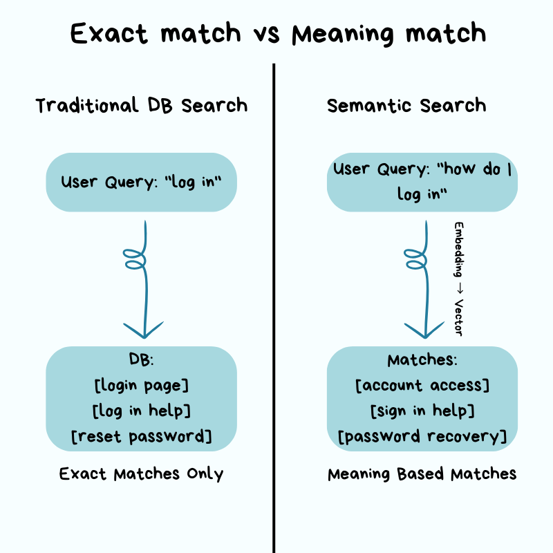
A user searching for “how do I log in” should find results about “account access” and “sign in” even if those exact words never appear in their query.
This kind of search, where the database understands meaning rather than just matching words, is called semantic search. It requires a completely different approach to how you store and search your data.
Yet if you try adding this in as a feature, everything that made your traditional relational database fast will stop working.
The tools you relied on: indexes, WHERE clauses, keyword matching were all built for finding exact values.
Semantic search does NOT work with exact values.
Instead, it works with meaning, and meaning is harder to search efficiently. A search that took milliseconds before now takes seconds, and the bigger your dataset, the worse it gets.
Your database is NOT broken.
It’s doing exactly what you told it to do: comparing your search against every single item in your database, one by one, because there is no other way to find “similar” when there is NO exact match.
This is where vector databases come in.
Not because they are trendy, but because traditional databases were never designed to handle this kind of search at scale.
If you’re a software engineer encountering the term “vector database” for the first time, whether your team is adding AI features or you keep seeing it mentioned everywhere and want to understand what it actually means, this newsletter explains it from the ground up…
[Webinar] Stop babysitting your coding agents (Partner)

Agents can generate code. Getting it right for your system, team conventions, and past decisions is the hard part – you end up wasting time and tokens in correction loops.
More MCPs give agents access to information, but not understanding. The teams pulling ahead use a context engine to give agents exactly what they need.
Join Unblocked live on May 6 (FREE) to see:
Where teams get stuck on the AI maturity curve
How a context engine solves for quality, efficiency, and cost
Live demo: the same coding task with and without a context engine
(Thanks to Unblocked for partnering on this post.)
I want to introduce Maxine as the guest author.

She’s a cloud infrastructure engineer who spends her days scaling databases, debugging production incidents at 2 am, and writing about what actually works in production.
You can get a copy of her LLMs for Humans: From Prompts to Production (at 30% off right now). It’s 20 chapters of practical applied AI with real production context, not theory. And it’ll help you get smarter about using AI tools in infrastructure workflows.
Checkout her work:
Plus, if you’re thinking about making a career move into cloud or DevOps and want a structured path to get there, get a copy of her The DevOps Career Switch Blueprint.
Inside this newsletter, you’ll get:
Why traditional search breaks. How exact-match databases fail with semantic meaning and why O(n) similarity search doesn’t scale.
How vector search works. Embeddings, high-dimensional space, and why similarity is measured by distance instead of exact matches.
The core architecture. Storage, indexing (HNSW), and query layers, with key tradeoffs in cost, latency, and accuracy.
Query execution in practice. ANN search, metadata filtering (pre vs post), and ranking, including how real systems return results.
Production realities. Scaling, replication, cost structure, monitoring, and failure modes teams hit in production.
Decision framework. When pgvector is enough, when to use a dedicated vector DB, and when distributed systems become necessary.
Why Traditional Databases Struggle with Embeddings
Traditional relational databases are good at exact matches and range queries.
They use indexes and data structures so the database can jump directly to relevant rows without scanning the entire table.
When you query WHERE user_id = 12345, database uses an index to find that row instantly, the same way you’d look up a word in a dictionary: you don’t read every page, you jump straight to the right section. Also when you query, WHERE created_at > ‘2026-01-01’, it works the same way for dates.
But embeddings break this model because there is no exact value to look up!
An embedding is a list of numbers that represents the meaning of a text.
Words, sentences, or entire paragraphs get converted into these numbers by an AI model, and similar meanings produce similar numbers.
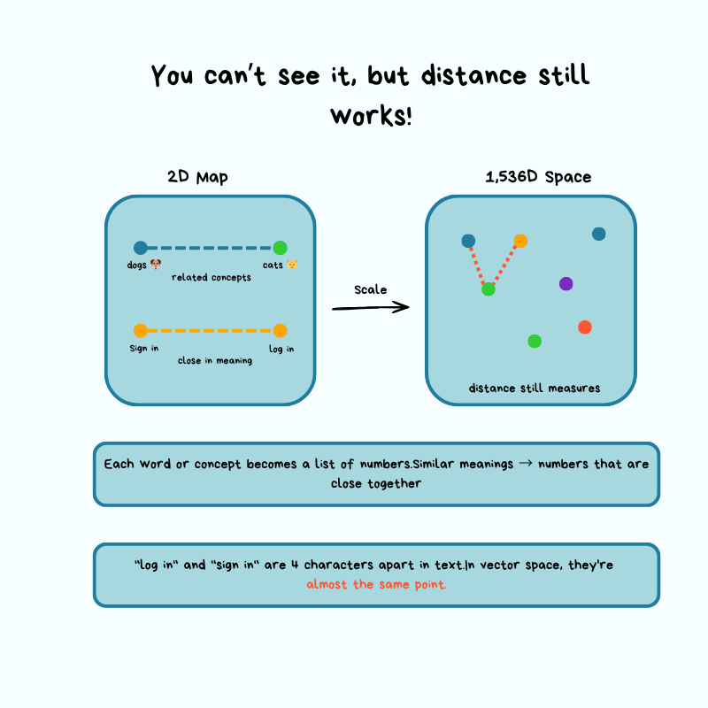
Instead of finding a specific row, you find rows closer in meaning, and “close” requires measuring distance in high-dimensional space rather than matching values. Think of it like a regular map with latitude and longitude, except you’re working with 1,536 dimensions instead of just 2.
Let’s walk through a concrete example to see why this creates a problem…
Imagine you have a document database where each document gets split into chunks.
And think of chunks like cutting a book into individual paragraphs so you can search each one separately. Each chunk gets converted into a 1,536-dimensional vector using an embedding model like OpenAI’s text-embedding-3-small:
A user submits a search query
App converts the query into a vector using the same embedding model
Now you have to find the “most similar” document chunks
Without specialized indexing, the only way to find “most similar” ones is to calculate the distance between your query vector and every chunk vector in your database, sort by distance, and return the top results.
Let’s break down what it means…
A vector is simply a list of numbers. In AI, those numbers represent meaning.
When you convert text into an embedding, you’re assigning it a location in a very high-dimensional space (imagine a map with 1,536 dimensions instead of the normal 2, latitude and longitude). Similar pieces of text end up close to each other on this map, while unrelated text ends up far apart.
When a user searches for something, their query also gets converted into coordinates on this map. To find the most relevant results, you need to measure the distance from the query’s location to every document chunk’s location in your database, then return the closest ones.
But here’s the problem…
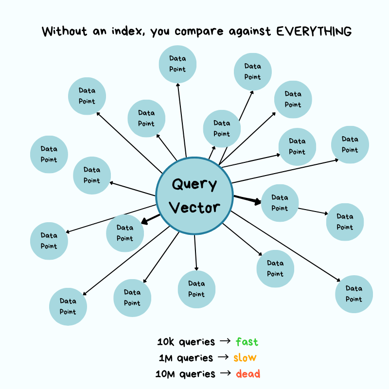
Without an index, there’s no shortcut. You must measure the distance to each item.
Now imagine you’re standing in Times Square in New York City, and you need to find the 10 closest coffee shops. Without a map or any organized system, your only option is to:
Walk to every building
Check if it’s a coffee shop
Measure how far it is from Times Square
Keep a list of the 10 closest ones you’ve found
If there are 10k buildings, you check all 10k. And if there are 10 million buildings, you check all 10 million.
The more buildings that exist, the longer it takes…
Put simply, it takes O(n) time, and it grows linearly with the size of your dataset.
In practical terms, if you have 10,000 document chunks and each distance calculation takes 0.0001 seconds, one query takes 1 second. That’s not terrible.
But what if you have 10 million chunks?
That same query now takes 1,000 seconds, i.e., 16 minutes. And if your application serves 100 queries per second from different users? Your system immediately grinds to a halt!
This is why traditional databases struggle with embeddings…
Their indexes are built for exact matches.
They can jump straight to user_id = 12345 without checking every row. But with vectors, there are no exact matches, only “similar” matches, and similarity requires measuring distances.
Let’s now imagine finding a similar song to the one you already like…
You cannot just look it up by name; you have to compare it against every other song across hundreds of characteristics: tempo, key, energy, mood, and so on. The more songs in your library, the longer it takes.
Vector search works the same way, except instead of songs, you compare text, and instead of a few characteristics, you are comparing across 1,536 dimensions at the same time.
Without specialized techniques to avoid checking everything, the math simply doesn’t scale.
This is where people often bring up pgvector, a PostgreSQL extension that adds vector search capabilities to Postgres. It’s a good option for smaller datasets and lets you avoid adding another database to your stack. This keeps operational efforts very low.
For datasets with fewer than 100,000 vectors and moderate query volumes, pgvector works well and keeps your infrastructure simpler.
But as your dataset grows into the millions and your query latency requirements tighten, you hit the limits of what a general-purpose database can do for this specific workload.
You don’t need a specialized vector database just because you’re working with embeddings, but you need to understand when the operational trade-offs tip in favor of dedicated infrastructure.
This brings us to the core challenge that vector databases solve…
How do you find approximate nearest neighbors in high-dimensional space without comparing against every vector, while still returning results that are “good enough” in terms of accuracy?
The answer involves building specialized index structures that trade accuracy for massive speed improvements, and understanding those trade-offs is essential for operating these systems in production.
Architecture: How It Works Under the Hood
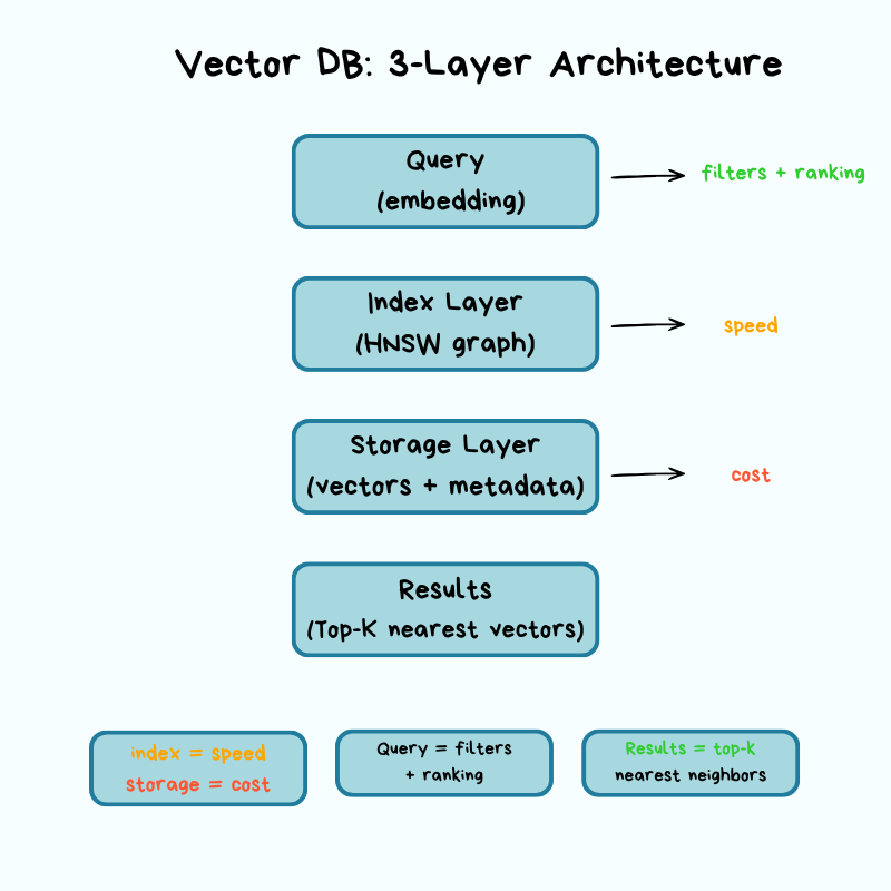
Vector databases have three key layers: storage, index, and query.
Each layer involves trade-offs that directly affect your operational concerns: cost, latency, accuracy, and scalability.
Let’s break down what matters from an infrastructure perspective…
Storage Layer: Where Vectors Live
Vectors are massive.
A single 1,536-dimensional vector using 32-bit floats takes up 6KB of storage. If you multiply that across millions of vectors, storage costs add up fast. This is a problem every vector database must solve at its foundation: the storage layer determines how vectors are physically stored, compressed, and retrieved from disk. This layer focuses on compression techniques that reduce both storage costs and the memory footprint while preserving as much accuracy as possible.
The most common approach is quantization.
Quantization reduces the precision of each dimension to use fewer bits.
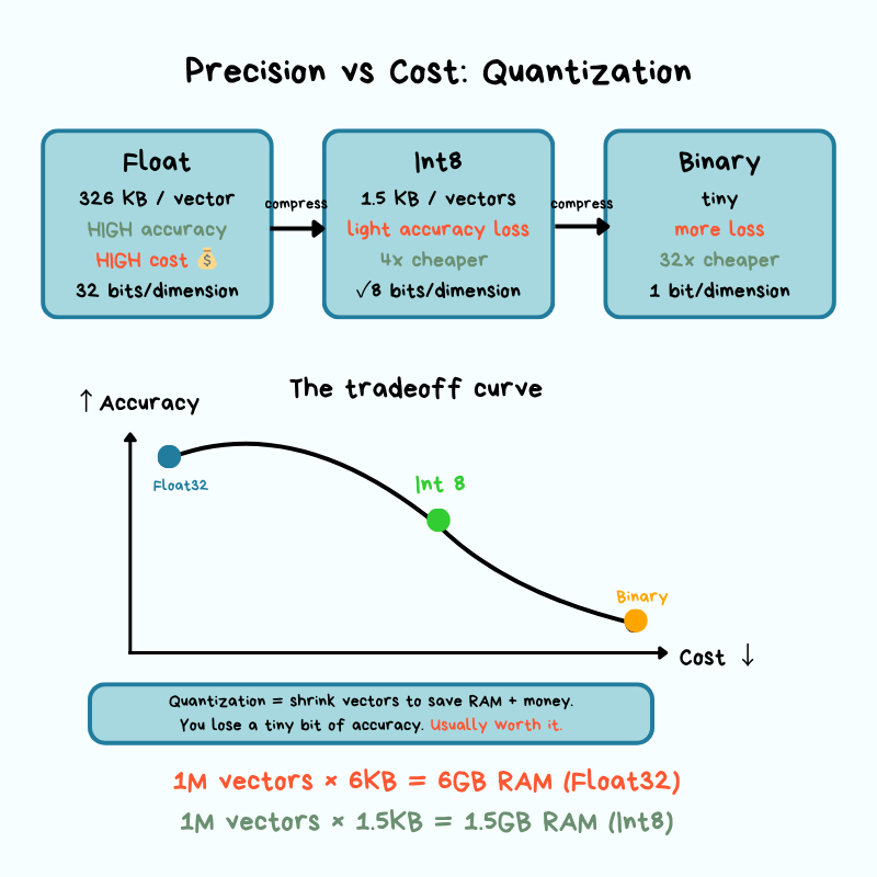
Instead of storing each dimension as a 32-bit float, you quantize to 8-bit integers (scalar quantization) or binary representations (binary quantization).
This can reduce storage and memory requirements by 4x or more, but it introduces approximation error. Approximation error is the gap between the compressed version of data and the original.
When you round numbers to save space, your calculations become slightly less precise. In vector search, this means you might occasionally miss a result that was truly the closest match, but in practice, the difference is small enough that most applications never notice it.
In production, you’re constantly trading off storage costs for search accuracy, and the right balance depends on your use case.
Another critical decision is the trade-off between memory and disk…
For maximum query speed, you want your vector index in memory, but that’s expensive at scale. Some vector databases support tiered storage, where frequently accessed vectors stay in memory while cold data lives on disk, or hybrid approaches in which the index structure stays in memory while raw vectors get pulled from disk when needed.
These architectural choices directly affect your cost structure and query latency percentiles.
From an operational perspective, you need to understand how your chosen vector database handles durability and recovery:
What happens if a node crashes mid-write?
How long does it take to rebuild indexes after a restart?
Are vectors written to disk synchronously or asynchronously?
These aren’t theoretical questions. They’re the difference between acceptable downtime and a major incident when something goes wrong.
Indexing Layer: Graph Structure
This is where the “magic” happens, and by magic I mean carefully engineered data structures that let you find approximate neighbors without exhaustive search.
The most popular algorithm in production vector databases is HNSW (Hierarchical Navigable Small World), and it’s worth understanding at a conceptual level even if you’re not implementing it yourself.
The core idea behind HNSW is based on “small world” networks, the same principle that says you’re only a few connections away from any other person on the planet.
Instead of comparing your query vector against every vector in your database, HNSW builds a multi-layer graph in which similar vectors are connected to each other. When you query, the algorithm starts at the top layer and navigates toward your target by following edges to similar neighbors, dropping through layers until it reaches the most similar vectors at the bottom layer.
Remember our map analogy?
Your vectors are locations on a high-dimensional map, and you’re trying to find the closest ones to your query without checking every single location. HNSW solves this by building a navigation system with different zoom levels.
Think of it like Google Maps navigating from New York to a specific coffee shop in San Francisco:
Top layer (zoomed out): From New York, HNSW identifies the general direction of your target, the West Coast, and follows connections to get you to California. You’re not considering every city in America, just the major waypoints that get you closer to where you need to be.
Middle layers (zooming in): Now you’re looking at California. The algorithm narrows down to the San Francisco Bay Area, following connections between nearby locations. You’re still not checking every street, just the neighborhoods that are directionally correct toward the coffee shop you want to visit.
Bottom layer (street level): Finally, you’re at the specific neighborhood and can see individual addresses. The algorithm follows the last few connections to find the exact coffee shop location (or, in vector terms, the most similar document chunks).
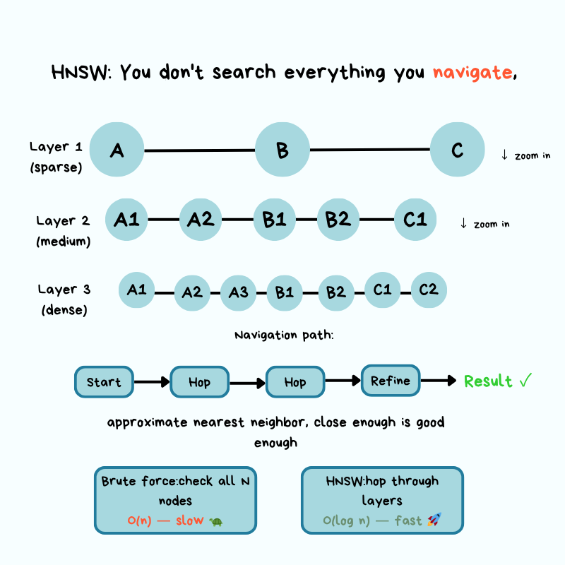
At each zoom level, you’re following connections between “nearby” locations without checking everywhere.
You only need to follow the connections that get you closer to your target. This is how HNSW turns an O(n) problem into something much faster: it builds a navigation structure that lets you skip large portions of the map in the wrong direction.
The key trade-off in HNSW is speed versus accuracy, controlled by two parameters: the number of connections each vector has (called “M” or “max connections”) and the number of neighbors to check during search (called “ef” or “exploration factor”).
Higher values mean better accuracy, but slower queries and larger indexes…
Lower values mean faster queries, but you might miss some relevant results. In production, you tune these parameters based on your latency requirements and tolerance for accuracy.
Building the HNSW index is expensive.
Inserting vectors requires calculating distances and updating graph connections, which is why bulk index building often happens offline or during low-traffic periods. Index build time matters because it affects how quickly you can recover from failures, deploy updates, or onboard new data.
You do not need to understand the math behind HNSW to work with vector databases.
Just like driving a car, you might not know how the engine works, and that doesn’t affect how you drive. But knowing that the engine exists and what it does helps you figure out what is wrong when the car breaks down.
What you need to know is that HNSW produces approximate results, not perfect ones, and it’s possible to adjust its approximation. When search results seem wrong, queries suddenly slow down, or the index fails to build, this understanding helps you identify the problem.
Get a copy of LLMs for Humans: From Prompts to Production right now and save 30%.

Reminder: this is a teaser of the subscriber-only newsletter, exclusive to my golden members.
When you upgrade, you’ll get:
High-level architecture of real-world systems.
Deep dive into how popular real-world systems work.
How real-world systems handle scale, reliability, and performance.
And much more!
Query Layer: How Requests Move Through System
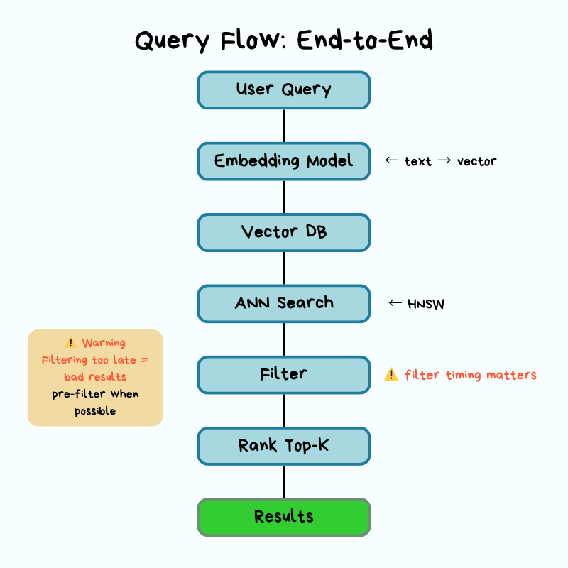
When a query hits your vector database, it follows a specific path:
Keep reading with a 7-day free trial
Subscribe to The System Design Newsletter to keep reading this post and get 7 days of free access to the full post archives.
 | A guest post by
|